Arps Equation: A Foundational Tool for Production Forecasting
The Arps equation stands as a cornerstone of oil and gas production forecasting, providing a relatively simple yet effective method for predicting well decline. For decades, it has served as a reliable tool for estimating future production, helping companies make informed decisions about resource allocation and future planning. However, understanding its strengths and limitations is crucial for accurate forecasting in today's complex energy landscape. This guide will explore the Arps equation, its applications, and limitations, and introduce more advanced techniques for enhanced accuracy. Are you ready to master this fundamental forecasting tool?
Diving Deep into the Arps Equation: Parameters and Decline Types
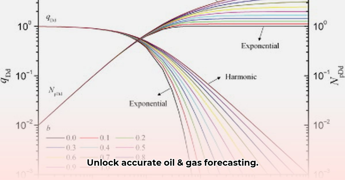
The Arps equation models the decline in production rate over time using two key parameters: the decline rate (D) and the exponent (b). The decline rate (D) represents the percentage decrease in production per unit of time. The exponent (b) determines the type of decline curve, influencing the shape of the production decline profile. Three primary decline types are modeled by the Arps equation:
Exponential Decline (b = 0): This type exhibits a constant percentage decline in production over time. Think of it as a consistent, predictable decay. (A simple, linear decrease in production)
Hyperbolic Decline (0 < b < 1): This is the most common decline type, characterized by a fast initial decline that gradually slows over time. (Production decreases rapidly initially, then at a slower rate)
Harmonic Decline (b = 1): This shows a decline that slows dramatically, with production rates diminishing more gradually than in hyperbolic decline. (The slowest rate of decline among the three)
To apply the Arps equation effectively, historical production data is necessary to determine the values of D and b, ultimately enabling the projection of future production rates. While the calculations themselves are relatively straightforward, numerous software packages and spreadsheets simplify the process. How many reservoir engineers are using spreadsheet software to perform these calculations?
Strengths and Limitations of the Arps Equation
The Arps equation's simplicity is both its greatest strength and its biggest weakness. Its ease of use makes it accessible to a wide range of professionals, contributing to its enduring popularity. However, its simplicity means it makes significant simplifying assumptions about the reservoir and its behavior.
Strengths:
- Ease of Use: Simple to understand and apply, requiring minimal computational resources.
- Wide Applicability (with caveats): Provides reasonable estimates for many conventional reservoirs.
- Established Baseline: Serves as a valuable benchmark for comparison with more advanced techniques.
Limitations:
- Simplified Reservoir Behavior: Doesn't fully capture the complexities of reservoir dynamics, such as fluid properties, pressure changes and heterogeneity.
- Inaccuracy in Unconventional Reservoirs: Struggles to accurately predict the production from unconventional reservoirs (e.g., shale gas) due to their complex flow dynamics.
- Data Dependency: Accurate forecasts rely heavily on accurate and complete historical production data. Poor data quality leads to significant prediction errors. According to Dr. Sarah Chen, Senior Reservoir Engineer at ExxonMobil, "The accuracy of decline curve analysis relies entirely on the quality of your input data."
Advanced Decline Curve Analysis Techniques: Moving Beyond the Arps Equation
While the Arps equation provides a useful starting point, more sophisticated techniques are required for greater accuracy, especially when dealing with unconventional reservoirs or complex reservoir behavior. These include:
Material Balance Analysis: This technique considers reservoir pressure, fluid properties, and volumes for a more comprehensive understanding of reservoir behavior. It provides a more holistic view than the well-centric approach of the Arps equation.
Reservoir Simulation: Powerful computer models that simulate reservoir behavior, considering numerous factors that the Arps equation simplifies or ignores. These models offer significantly enhanced accuracy but require significant computational resources.
Artificial Intelligence (AI) and Machine Learning (ML): Data-driven approaches using AI and ML algorithms can analyze massive datasets to identify patterns and relationships beyond the capabilities of simpler techniques. This holds considerable promise for enhancing prediction accuracy, particularly for unconventional resources. "Machine learning offers the potential to revolutionize decline curve analysis," notes Dr. David Lee, Professor of Petroleum Engineering at Stanford University.
Data Quality: The Foundation of Accurate Forecasting
The accuracy of any forecasting model, including the Arps equation and its advanced counterparts, is fundamentally dependent on the quality of the input data. Inaccurate or incomplete data will inevitably lead to poor predictions. Therefore, robust data acquisition, cleaning, and quality control processes are crucial for reliable forecasting. This includes:
- Reliable Data Sources: Utilizing data from multiple sources to ensure consistency and completeness (well tests, SCADA systems, seismic surveys, etc.).
- Data Cleaning and Validation: Implementing rigorous quality control measures to identify and correct errors. This crucial step significantly improves forecast accuracy.
- Data Integration: Combining different datasets to create a more comprehensive picture of the reservoir’s behavior.
Actionable Steps for Stakeholders: Improving Forecasting Processes
To maximize the effectiveness of decline curve analysis, various stakeholders need to take specific actions:
Oil & Gas Companies: Invest in robust data management systems and integrate advanced analytics into their decision-making processes. This includes training and development programs for employees in the latest forecasting techniques.
Reservoir Engineers: Leverage their expertise to select the most appropriate forecasting model, refining data quality procedures and utilizing advanced analysis tools.
Production Managers: Utilize improved forecasts to optimize production schedules, allocate resources effectively, and proactively adjust operations to maximize profitability.
Data Scientists: Develop and refine sophisticated forecasting models using AI and ML, focusing on data integration and improving overall accuracy.
Implementing these steps will greatly improve the accuracy and reliability of production forecasting.
Conclusion: A Holistic Approach to Production Forecasting
While the Arps equation remains a valuable tool due to its simplicity and ease of use, a more comprehensive and integrated approach combining it with advanced techniques is necessary for accurate production forecasting, especially in complex scenarios and unconventional reservoirs. This involves leveraging the power of advanced analytics, AI, machine learning, and rigorous data quality control. By embracing this holistic approach, oil and gas companies can improve their decision-making, optimize resource allocation, and ensure long-term operational success.